Markov Chain Monte-Carlo... in Swift
"All models are wrong, and increasingly you can succeed without them" - Peter Norvig
If you want to test the code on your side, you can go on the github notebook and execute the code in a google colab notebook
One of my motivation of coding from scratch is to grasp the concepts which can be very abstract when we stick to the formulas, this algorithm is not new and my article won't be the last one on the topic, my hope is to bring another angle of understanding to this topic which is often either too simplified or too formally explained. I'd be pleased to have some reviews in the comments section.
A few notions of MCMC and Metropolis-Hastings
Metropolis-Hasings algorithm allows us to sample from a generic probability distribution (we'll call it target distribution $p$) event if we don't know our normalizing constant $p(D)$ or $p(x)$ with $x$ representing our data.
To do this, we'll build and sample from a Markov Chaine who's distribution will be the target distribution we're looking for.
Let's remind the bayes formula and the terms to be well understood : $$ p(\theta | X) = \frac{p(X|\theta)p(\theta)}{p(X)} = \frac{p(X|\theta)p(\theta)}{\int_\Theta p(X|\theta)p(\theta)d\theta} $$ with :
Now that we reminded the basic formula, we can now go on to Markov Chains explanation, the goal of such a method and the constraints that lead us to use the Metropolis-Hasings algorithm.
Markov Chain consists of :
Here, we want to produce samples from a target distribution $p$ but we only know it on a certain proportion : We don't know the normalizing constant $p(X)$ because it would be difficult to integrate so we only have a distribution $g$ which is proportional to $p$ or simply $g \propto p$ to work with.
The Metropolis-Hastins algorithm step-by-step and intuition behind the algorithm:
(1) - Select an initial value of $\theta_0$
(2) - For $i = \{1,...,N\}$, with $N \in \mathbb{N}$
a) Draw a candidate parameter $\theta^*$ from a proposal distribution $q(\theta^*|\theta_{i-1})$
b) Next, we compute a ratio $\alpha = \frac{g(\theta^* | X)q(\theta_{i-1} | \theta^*)}{g(\theta_{i-1} | X)q(\theta^* | \theta_{i-1})} = \frac{g(\theta^* | X)}{g(\theta_{i-1} | X)}$(*)
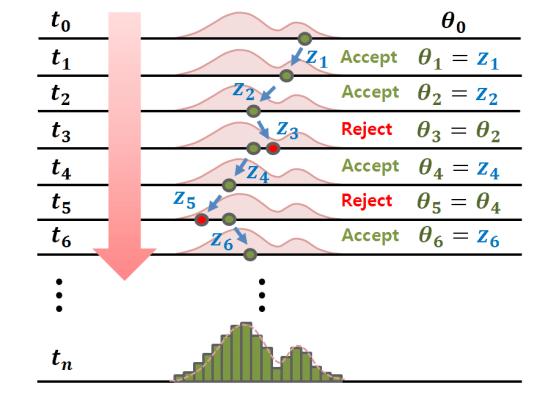
c) - If $\alpha \geqslant 1$ : accept $\theta^*$ and set $\theta_i = \theta^*$
- Else if $0 < \alpha < 1$ : accept $\theta^*$ and set $\theta_i = \theta^*$ with probability $\alpha$
reject $\theta^*$ and set $\theta_i = \theta_{i-1}$ with probability $1 - \alpha$
The steps b) and c) act as a filter of the sampled candidates, since the proposal distribution $q$ is not the target distribution $p$
At each step in the chain, we draw a candidate $\theta^*$
and decide whether to move in the chain (assign a new value $\theta^*$ to $\theta_i$)
there or to remain where we are (keep the same value by assigning $\theta_{i-1}$ to $\theta_i$) :
Since our decision to move to the candidate only depends on where the chain currently is, we verify the property of the Markov Chain.
One careful choice we'll make is on the choice of the proposal distribution or candidate generating distribution $q(\theta^*|\theta_{i-1})$ as it may or may not depend on the previous value of $\theta$.
ex: Where it doesn't depend on the previous value :
--> if $q(\theta^*)$ is always the same distribution, then $q(\theta)$ should be similar to $p(\theta)$ to approximate it.
ex 2: Where it does depend on the previous value : Random walk metropolis-hastings
--> The proposal distribution $q$ is centered on the previous iteration $\theta_{i-1}$. It might be a Normal distribution where the mean is our previous iteration parameter $\theta_{i-1}$.
Because the Normal distribution is symetric around its mean, this example comes with a nice advantage with : $q(\theta^* | \theta_{i-1}) = q(\theta_{i-1} | \theta^*)$
It causes the ratio $\alpha$ to be simplified to : $\alpha = \frac{g(\theta^* | X)}{g(\theta_{i-1} | X)}$(*)
This case is generally the most used and we will develop this part, we can sum up our step-by-step algorithm with both of the following illustrations :
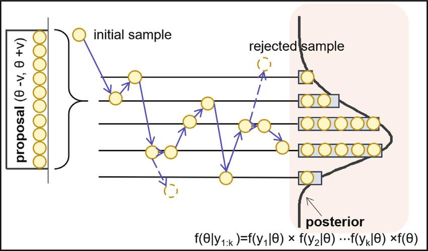
As explained before and to sum up to our approach, our proposal distribution ($q$) is centered on the $\theta$ value which depends on the acceptance or rejection decision of the previous iteration with a variance $v$
Then we stack the accepted parameters $\theta$ to create our posterior distribution by accepting or rejecting them conditioned on the data $y_{1:k} = \{y_1,...y_k\}$
Practical application on synthetic data :
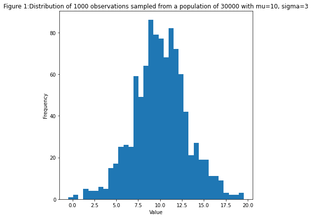
We generate a large amount of samples from a normal distribution with $\mu = 10$ and $\sigma = 3$, but we only observe 1000 samples.
import Foundation
import Darwin
import Python

%include "EnableIPythonDisplay.swift"
IPythonDisplay.shell.enable_matplotlib("inline")

let plt = Python.import("matplotlib.pyplot")

...

let mod1 = Normal(mean: 10, sd: 3).random
let population = mod1(30000)

let index_shuffled = (0..<30000).shuffled()[0..<1000]
var observations:Array<Double> = []


for i in index_shuffled {
    observations.append(population[i])
}

let fig = plt.figure(figsize:[7,7])
let ax = fig.add_subplot(1,1,1)
ax.hist(observations, bins:35)
ax.set_xlabel("value")
ax.set_ylabel("Frequency")
ax.set_title(Figure 1:Distribution of 1000 observations sampled from a population of 30000 with mu=\(mean_), sigma=\(sd_)")
plt.show()
Objective and what we're looking to solve:
To make it simple, we'd like to find a distribution for $\sigma_{obs}$ using the 1000 observed samples. In this problem we're looking for sampling the parameter $\sigma$ so it may be rather simple but for real applications,
it's gonna be also about finding the distributions of the parameters of a unimodal or multimodal distribution.
Definition of the proposal distribution :
We don't have any idea for a probabilistic distribution so we're gonna just choose a simple and symetric one like we said in the 2nd example above : a Normal distribution. $$Q(\sigma^* | \sigma_{actual}) \sim \mathcal{N}(\mu = \sigma_{actual}, \sigma' = 0.5)$$ Where $\sigma'$ is not related to either $\sigma^*$ nor $\sigma_{actual}$ with $\sigma_{actual} = \sigma_{i-1}$. We'll draw 1 sample $\sigma^*$ from this Normal distribution.The proposal distribution will be called transition model to make it more intelligible when reading the code.
Definition of the likelihood :
As a reminder, we said that we don't know the exact formula for the posterior distribution $p(\theta | X)$ but only the approximate one $g(\theta | X)$ which can be expressed the following way : $$g(\theta | X) \propto g(X | \theta)g(\theta)$$ with:In order to express the likelihood, we have to know the probability density that fits the best to the distribution of our data. Or in a more mathematically correct way, we have to find a distribution which is proportional to the posterior, we then define for each data point $x_i$ in the data $X$. In our case, we'll choose a Normal distribution density function with : $$f(x_i | \theta) = \frac{1}{\sqrt{2\pi\sigma^2}}e^-{\frac{(x_i - \mu)^2}{2\sigma^2}}$$ where:
The likelihood is the defined as : $$g(X | \theta) = \Pi_{i}^{n}f(x_i | \theta)$$ This formula will be useful to define the calculation of our ratio $\alpha$.
Acceptance/Rejection conditions :
The acceptance/rejection conditions will be based on the calculation of the following ratio : $$\alpha = \frac{g(\theta^* | X)}{g(\theta_{i-1} | X)} = \frac{g(X | \theta^*)g(\theta^*)}{g(X | \theta_{i-1})g(\theta_{i-1})}$$- If $\alpha$ is larger than the random number generated, then we accept $\sigma^*$.
- Otherwise, we reject $\sigma^*$ and keep the last iteration value by assigning $\sigma_{i} = \sigma_{i-1}$
Definition of the Prior and log-likelihood for the calculation the ratio :
As we mentioned before, the likelihood for the data/the observation $X$ is : $g(X | \theta) = \Pi_{i}^{n}f(x_i | \theta)$ We'll take the log-likelihood instead of the likelihood because of a computation matter : The computation cost is more important for a multiplication rather that an addition of batch of values.Remember, the condition we accept our rate $\alpha$ is when it is above 1, then we can write : $$\frac{g(X | \theta^*)g(\theta^*)}{g(X | \theta_{i-1})g(\theta_{i-1})} > 1$$ $$log(\frac{g(X | \theta^*)g(\theta^*)}{g(X | \theta_{i-1})g(\theta_{i-1})}) > 0$$ $$log(g(X | \theta^*)g(\theta^*)) - log(g(X | \theta_{i-1})g(\theta_{i-1})) > 0$$ $$log(g(X | \theta^*)g(\theta^*)) > log(g(X | \theta_{i-1})g(\theta_{i-1}))$$ $$log(g(X | \theta^*)) + log(g(\theta^*)) > log(g(X | \theta_{i-1})) + log(g(\theta_{i-1}))$$ $$\Sigma_{i}^{n}log(f(x_i | \theta^*)) + log(g(\theta^*)) > \Sigma_{i}^{n}log(f(x_i | \theta_{i-1})) + log(g(\theta_{i-1}))$$ $$\Sigma_{i}^{n}log(\frac{1}{\sqrt{2\pi\sigma^{*2}}}e^-{\frac{(x_i - \mu)^2}{2\sigma^{*2}}}) + log(g(\theta^*)) > \Sigma_{i}^{n}log(\frac{1}{\sqrt{2\pi\sigma_{i-1}^{2}}}e^-{\frac{(x_i - \mu)^2}{2\sigma_{i-1}^{2}}}) + log(g(\theta_{i-1}))$$ We carefully take note that $\mu$ is constant ! As we try to sample the distribution of $\sigma$, we obtain the acceptance condition we'll compute : $$\Sigma_{i}^{n}(log(\sigma^*\sqrt{2\pi}) - \frac{x_i - \mu}{2\sigma^{*2}} ) + log(g(\theta^*)) > \Sigma_{i}^{n}(log(\sigma_{i-1}\sqrt{2\pi}) - \frac{x_i - \mu}{2\sigma_{i-1}^{2}} ) + log(g(\theta_{i-1}))$$ We won't reduce any longer to make the computation code easy to read.
For our prior distribution, the only constraint we have is that $\sigma > 0$, we could choose to model it with a Half-normal distribution or any positive function but to make it simple, we'll just put a condition so that if the standard deviation is negative, then we'll just put the log to $-\infty$ which will lead to a rejection of the sample or make it equal to 1 in order to cancel the log and have a simpler calculation.
Let's now Implement our Metropolis-Hastings algorithm :
Metropolis-Hastings algorithm - Swift implementation :
func transition_model(_ x:Array<Double>) -> Array<Double> {
    var ret_arr:Array<Double> = []
    ret_arr.append(x[0])
    ret_arr.append(Normal(mean: x[1], sd: 0.5).random(1)[0])
    return ret_arr
}

func prior(_ x:Array<Double>) -> Int {
    if (x[1] <= 0) {
        return 0
    }
    return 1
}

func manual_log_like_normal(_ x:Array<Double>,_ data:Array<Double>) -> Double {
    let fact_1:Double = -log(x[1] * pow(2 * Double.pi, 0.5))
    let fact_2:Array<Double> = data.map({pow($0 - x[0],2) / (2 * pow(x[1],2))})
    var substract:Array<Double> = []
    for i in 0..< fact_2.count {
        substract.append(fact_1 - fact_2[i])
    }
    return (substract).reduce(0,+)
}

func acceptance(_ x:Double, _ x_new:Double) -> Bool {
    if x_new > x {
        return true
    }
    else {
        let accept:Double = Uniform(a: 0, b: 1).random(1)[0]
        return (accept < (exp(x_new - x)))
    }
}

func metropolis_hastings(_ likelihood_computer:(_ x:Array<Double>,_ data:Array<Double>) -> Double,_ prior:(_ x:Array<Double>) -> Int, _ transition_model:(_ x:Array<Double>) -> Array<Double>, _ param_init:Array<Double>,_ iterations:Int,_ data:Array<Double>,_ acceptance_rule:(_ x:Double, _ x_new:Double) -> Bool) -> ((Array<Double>,Array<Double>), (Array<Double>,Array<Double>)) {
    var x:Array<Double> = param_init
    var accepted:(Array<Double>,Array<Double>) = ([],[])
    var rejected:(Array<Double>,Array<Double>) = ([],[])
    for i in 0..< iterations {
        var x_new:Array<Double> = transition_model(x)
        var x_lik:Double = likelihood_computer(x, data)
        var x_new_lik:Double = likelihood_computer(x_new, data)
        if acceptance_rule( x_lik + log(Double(prior(x))), x_new_lik + log(Double(prior(x_new))) ) {
            x = x_new
            accepted.0.append(x_new[0])
            accepted.1.append(x_new[1])
        }
        else {
            rejected.0.append(x_new[0])
            rejected.1.append(x_new[1])
        }
    }
    return (accepted, rejected)
}
Let's run the algorithm and get the accepted samples, we'll initialize our values with $\mu_{0} = \mu_{obs} = 10$ and $\sigma_0 = 0.1$ :
var accepted_rejected:((Array<Double>,Array<Double>),(Array<Double>,Array<Double>)) = (([],[]),([],[]))

accepted_rejected = metropolis_hastings(manual_log_like_normal,prior,transition_model,[mu_obs,0.1], 50000,observations,acceptance)
Over 50000 draws, 8465 samples were accepted which represent ~20.4% of accepted samples which is not bad.
One way to see if our algorithm is not doing well is if it's acceptance ratio is either too high or too low.
A good acceptance rate is generally between [20%...50%].
Now let's plot the results of our sampling :
let fig = plt.figure(figsize:[10,10])
let ax = fig.add_subplot(2,1,1)

ax.plot((0..<50).map({$0}), Array<Double>(accepted_rejected.1.1[0..<50]), "rx",label:"Rejected",alpha:0.5)
ax.plot((0..<50).map({$0}), Array<Double>(accepted_rejected.0.1[0..<50]), "b.",label:"Accepted",alpha:0.5)
ax.set_xlabel("Iterations")
ax.set_ylabel("sigma")
ax.set_title("Figure 2: MCMC sampling for sigma with Metropolis-Hastings. First 50 samples are shown.")
ax.grid()
ax.legend()

let ax2 = fig.add_subplot(2,1,2)
var to_show = accepted_rejected.0.1.count
var borne_max = accepted_rejected.1.1.count
var borne_min = borne_max - to_show

ax2.plot((0..< accepted_rejected.0.1.count).map({$0}), Array<Double>(accepted_rejected.1.1[borne_min..< borne_max]),"rx", label:"Rejected",alpha:0.5)
ax2.plot((0..< accepted_rejected.0.1.count).map({$0}), Array<Double>(accepted_rejected.0.1),"b.", label:"Accepted",alpha:0.5)
ax2.set_xlabel("Iteration")
ax2.set_ylabel("sigma")
ax2.set_title("Figure 3: MCMC sampling for sigma with Metropolis-Hastings. All samples are shown.")
ax2.grid()
ax2.legend()
plt.show()
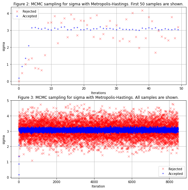
Not badly we see our algorithm converges well to the true value of $\sigma$ in blue we see the accepted samples and in red the rejected ones.
Next, we'll model only the accepted samples and the distribution of the accepted samples to have a credibility interval on our parameter $\sigma$
let show = Int(Double(accepted_rejected.0.0.count) * 0.75)

let fig = plt.figure(figsize:[20,10])
var ax = fig.add_subplot(1,2,1)
ax.plot((0..<(accepted_rejected.0.1.count - show)).map({$0}),Array<Double>(accepted_rejected.0.1[show..< accepted_rejected.0.1.count]))
ax.set_title("Figure 4: Trace for sigma")
ax.set_ylabel("sigma")
ax.set_xlabel("Iteration")
ax = fig.add_subplot(1,2,2)
ax.hist(Array<Double>(accepted_rejected.0.1[show..< accepted_rejected.0.1.count]), bins:20, density:true)
ax.set_ylabel("Frequency (normed)")
ax.set_xlabel("sigma")
ax.set_title("Figure 5: Histogram of sigma")

plt.show()
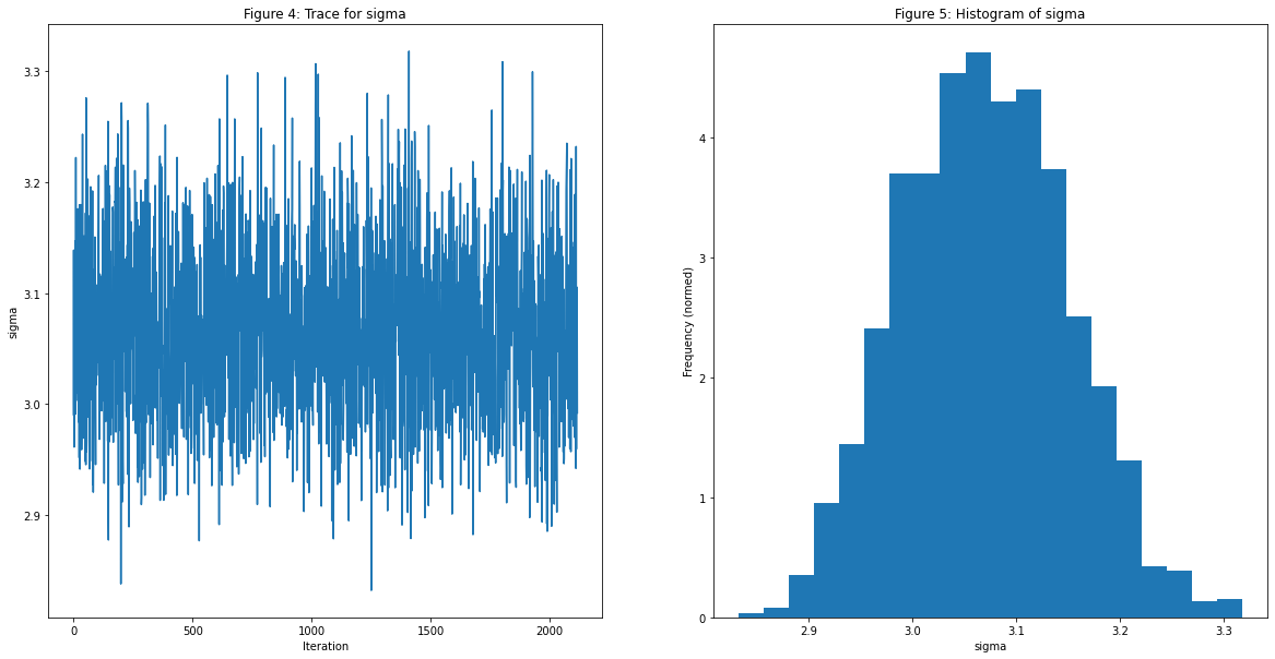
The values of $\sigma$ is concentrated between $[2.8,3.3]$ by only observing 1000 points out of the 30000 from $X$ which explains the uncertainty in our MCMC sampling.
Last checkup :
Now let's check that the sampled parameters will approximate well our distribution at the beginning by taking the mean of all parameters and generating data points with $\sigma$ as the mean of the posterior distribution generated through our MCMC sampling.let mu = Tensor<Double>(accepted_rejected.0.0[show..< accepted_rejected.0.0.count]).mean()
let sigma = Tensor<Double>(accepted_rejected.0.1[show..< accepted_rejected.0.1.count]).mean()
func model_lambda(_ t:Int,_ mu:Double,_ sigma:Double) -> Array<Double> {
let ret_val:Array<Double> = Normal(mean: mu, sd: sigma).random(t)
return ret_val
}
let observation_gen = model_lambda(population.count, Double(mu)!, Double(sigma)!)
let fig = plt.figure(figsize:[7,7])
var ax = fig.add_subplot(1,1,1)
ax.hist(observation_gen, bins:70, label:"Predicted distribution of 30,000 individuals")
ax.hist(population, bins:70, alpha:0.5, label:"Original values of the 30,000 individuals")
ax.set_xlabel("Mean")
ax.set_ylabel("Frequency")
ax.set_title("Figure 6: Posterior distribution of predictions")
ax.legend()
plt.show()
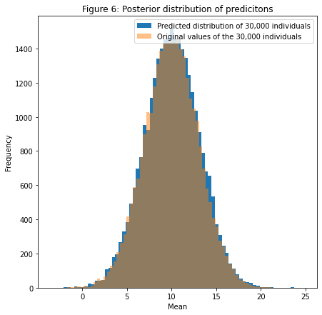
Great! We see now by taking the mean of our posterior distribution we could generate a distribution which is pretty close to our original distribution! In order to check for how good this prediction is, we'll have to implement an indicator called ELBO in order to quantify how our prediction fits the original data by using Expectation Maximization algorithm to find a lower bound of how "likely" our prediction is compared to other predictions. This will be for another article.