Gaussian Mixture Model - EM Algorithm

Expectation Maximization from scratch in Swift

---

"The only way to learn a new programming language is by writing programs in it" - Dennis Ritchie

---

This project work was inspired from Ritchie Vink for his article on GMMs and Alexander Tar thanks to its Swift implementation of statistical library
If you want to test the code on your side, you can go on the github notebook and execute the code in a google colab notebook

The Swift programming language

As the quote mentions, the aim of this project is both to improve my skills in data science by getting head-first in the algorithm we use every day to implement more complex code and also to learn a brand new language getting more and more famous : Swift.

One may wonder why Swift ? When we mention this language we first think about iOS application development so why getting into this language rather than Julia or even the classic ones Java/C++ which are already used in the industry for years ?
To make it short, Swift has 3 advantages that made me choose to get into this language rather than more recent ones (Julia) or older ones (C++):
    1 - The language is compiled and offers great performances close to C language.
    2 - The readability of the language is great compared to C++ or related.
    3 - The support of great industries like Google (with Swift for TensorFlow) and Apple to make improvement in this language compared to more open source languages like Julia which are great but don't have as much support from the industry as the Swift language may have.

To get more information on why this language may be great to learn and have some more details, I'll redirect you to the comprehensive article written by Jeremy Howards on this topic and his projection to improve his future deep learning framework through this language

Gaussian Mixture model

My goal is to give more explainability to the use of data science models. For this project, we are interested in the topic of unsupervised learning. If we are initiated to the machine learning area, the first thing that comes to our mind when talking about machine learning algorithm for unsupervised learning tasks are K-means, Density (DBSCAN) or mean shift algorithms.
The Issue with such topics is about how to give a boudary to the uncertainty of the clusters found by our algorithm ? How uncertain is our result ? Especially in unsupervised learning we need more to give us more confidence if we don't have any labels in our datasets.

We'll expose the problem through the clustering of a gaussian mixture model with the use of Expectation Maximization algorithm.
For the sake of simplicity, this project was made on 1D, in a next project, I'll use a general case with a multivariate distribution but it can take a little more time as it's done in Swift and not in Python.

---

The problem to solve is to decompose a probability distribution with several Gaussian distributions. Here we have an example of mixture model :

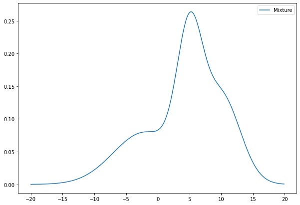
This distribution has been created by summing 2 Normal distributions, the aim of the algorithm is to find out these distributions and their parameters. The aim of our GMM is to model a probability distribution with several Gaussian distributions.
The most natural distribution we'll use to decompose this curve with is the Normal distribution, from there, we'll need an algorithm to infer these parameters :
This is where we'll introduce the Expectation Maximization algorithm

We assume a generative process where $X$ is the observed data corresponding to the data we want to fit the model on.
$z_i$ is the hidden random variable (aka latent but let's keep it easy here) that determines from which gaussian $i = \{1,...,m\}$, $m \in \mathbb{N}$ the observed data $x_k$ has been sampled from (where $k \in \mathbb{N}$ is the index of sample of the observed random variable $X$).

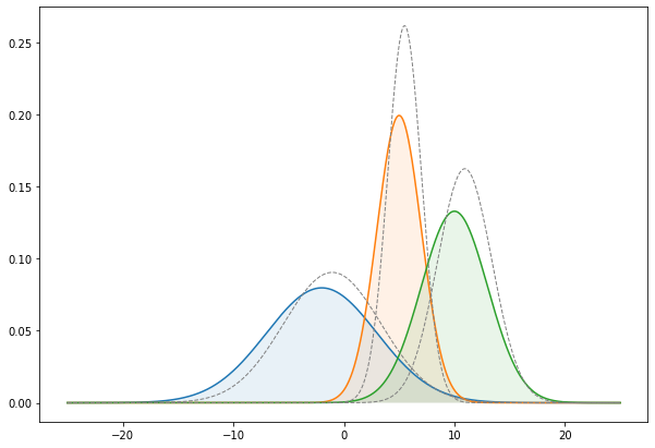
Below you'll see the 3 Gaussian curves from which we created the distribution to fit :

From there, we'd like to know what are the parameters of these gaussian distributions where for each gaussian $i$ : $$x_k|z_i \sim \mathcal{N}(\mu_i, \sigma_i^2)$$ Where $z_i = \left\{ \begin{array}{ll} 1 & \mbox{if $x_k$ belongs to gaussian $i$} \\ 0 & \mbox{otherwise.} \end{array} \right. $ then the distribution of $z_i$ would be :

$z_i \sim \mathcal{B}(n,p)$ in case of 2 gaussians

or $z_i \sim \mathcal{M}(n, \phi)$ for $i$ > 2 (for more than 2 gaussians)

with :

$\phi = \{\phi_1,...,\phi_m\}$ is a vector of probability for each possible $m$ outcome (gaussian distribution)

$\phi_i = p(z_i = 1)$ where $\phi_i$ corresponds to the probability of $z_i$ to be equal to 1 (that the gaussian selected is the $i$-th one).

$n \in \mathbb{N}^*$ corresponds to the number of trials.

For our example, we'll have 3 gaussians with $m = 3$.
The Swift code for this part :

You may wonder why we use Swift arrays instead of Python if we still use matplotlib. The reasons are because Python arrays are considered as "Python object" in Swift, so the interoperability is still limited. The second reason being that Swift objects are potentially way faster that Python objects which are just "references" to C code but not "value" objects, if you want more information between the difference between reference vs value types go check this link

Expectation Maximization

The aim of this algorithm is to find a local maximum likelihood or maximum a posteriori (MAP) estimates of parameters in the statistical model (Here a Gaussian mixture model). Our GMM depends on unobserved latent parameters (named $Z$) which are the parameters of the gaussians composing the mixture. And therefore, we'd like to find the optimal values of theses latent parameters to fit the gaussians which makes our model. But as we don't know the number of gaussians, $z_i$ is hidden and unknown so the likelihood has no known equation/known form.
For 1 gaussian, the maximum likelihood would be : $L(\theta;X)=L(\theta;x_1,...x_N) = f(x_1;\theta) \times ... \times f(x_N;\theta) = \prod_{k=1}^{N} f(x_k;\theta) = \prod_{k=1}^{N} p(x_k|\theta) $

with : $\theta = \{\mu, \sigma \}$ being shortcut for the parameters to estimate.

Yet here we clearly have a multimodal distribution so just solving the maximum likelihood would not fit our observed data very well.
In order to fit it, we need to solve the values of another random variable $Z$ which would give us the number of gaussians and find its associated parameter $\phi$
From there, our set of parameters to optimize for the solving of maximum likelihood becomes : $\theta : \{ \mu, \sigma, \phi \}$
And our likelihood function becomes : $L(\theta;X,Z) = P(X,Z|\theta)$
To find the maximum likelihood estimate, we'll then maximize the marginal likelihood of the observed data : $L(\theta;X) = p(X | \theta) = {\displaystyle \int }p(X,Z|\theta)dZ$
Where $L(\theta;X) = P(X | \theta) = {\displaystyle \prod_{k=1}^{N} }P(x_k|\theta) = {\displaystyle \prod_{k=1}^{N} } {\displaystyle \int_{z} }p(x_k, z | \theta) dz = {\displaystyle \prod_{k=1}^{N} } {\displaystyle \int_{z} }p(x_k| z, \theta)p(z|\theta) dz$ In our case, $Z$ is discrete so we'll rewrite the equation : $$L(\theta;X) = {\displaystyle \prod_{k=1}^{N} }{\displaystyle \sum_{i=1}^{m} }p(x_k|z_i, \theta)p(z_i|\theta) $$ And if we take the log of the expression, we get the log-likelihood expression we want to maximize : $$l(\theta;X) = log(L(\theta;X)) = {\displaystyle \sum_{k=1}^{N} }log ({\displaystyle \sum_{i=1}^{m} }p(x_k|z_i,\theta)p(z_i|\theta))$$ From this expression we know :

$x_i$ which is our $i$-th observed data (fixed because we marginalized out $Z$)

$\theta_0$ the set of parameters at the beginning or $\theta^{(t)}$ which is the set of updated parameters at iteration $t$

We know how many $z_i$ we want to "cluster" our multimodal distribution with gaussians

Yet, we don't know much on our gaussians! What are the true parameters $\theta$ for each gaussians $z_i$ ? Parameters also depends on the observation $X$.

In order to solve this issue the intuition is the following, we'll loop for $i = 1..n$ (number of gaussians) :
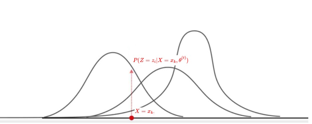
        1 - We weight the GMM likelihood by multiplying it by $P(Z = z_i | X = x_k, \theta^{(t)})$, the gaussian distribution $z_i$ conditioned by our observations $x_k$ and parameters $\theta$
        2 - We calculate the mean of the "weighed likelihood" with conditional expectation $E_{Z|X,\theta}[...]$ which will correspond to a (local) maximum because the log-likelihood is a concave function.
        3 - With the knowledge of the precedent values, we update the parameters values $\theta^{(t)}$ at iteration $t$ for the gaussian $z_i$ until one or several parameter of $\theta^{(t)} \leq \theta_{new} + \epsilon$ with a manually configured threshold $\epsilon$ which will define the "convergence" of the sampling of the gaussian parameters
Then loop to the next $i$

We can illustrate what we said before with the following illustration which shows for 1 loop at 1 point $x_k$ :


We'll use the EM algorithm to infer the value of the hidden random variable $Z$ (in other words, infer how probable is each gaussian $z_i$ with the parameters $\theta$ on the observed data $x_k$) through an iterative procedure by changing the parameter's values $\theta$ at each iteration :

Expectation step:

We are trying to compute the expected value of the log-likelihood function of $\theta$ conditionned to the distribution of $Z|X,\theta$ which is expressed by the auxiliary function $Q(\theta|\theta^{(t)})$: $$Q(\theta|\theta^{(t)}) = E_{Z|X,\theta^{(t)}}[l(\theta;X)] = E_{Z|X,\theta^{(t)}}[log(L(\theta;X))] = {\displaystyle \sum_{Z}}p(Z|X,\theta^{(t)})log(L(\theta;X))$$ $$Q(\theta|\theta^{(t)}) \approx {\displaystyle \sum_{Z}}p(Z|X,\theta^{(t)})log(L(\theta;X)),\quad log(L(\theta;X)) < 0$$

We don't know how negative our log-likelihood is as it's a distribution but we can have an idea of its average value over our latent variable $Z$ conditioned to $X$ and $\theta^{(t)}$ thanks to $p(Z|X,\theta)$

$w_{ij} = p(z_i|x_k,\theta) \propto p(x_k | z_i, \theta)p(z_i|\theta)$, we answer the questions :
"What is the likelihood the selected gaussian is the a priori $i$-th one knowing the observed data $x_k$ for a fixed set of parameters $\theta$ ?" or
"What is the a posteriori probability the gaussian selected is the $i$-th one conditioned on the observed data $X$ and the fixed parameters $\theta$?"

Maximization step:

We try to find the parameters that maximizes the parameters $\theta$ through an iterative algorithmic step to maximize the following quantity : $$\theta^{(t+1)}=argmax_{\theta}[Q(\theta|\theta^{(t)})]$$ We'll use all the data point to determine the new parameters

Concretely, we'll update each of the parameters of our $\theta$ : $$\phi_j := \frac{1}{n}\sum_{i=1}^n w_{ij}$$ $$\mu_j := \frac{\sum_{i=1}^nw_{ij} x_i} {\sum_{i=1}^nw_{ij}}$$ $$\sigma_j := \sqrt{\frac{\sum_{i=1}^nw_{ij}(x_i - \mu_j)^2} {\sum_{i=1}^nw_{ij}}}$$ We'll iterate until we get under a certain threshold from which we'll consider our algorithm has converged (hoping it would be the maximum likelihood).

Nota Bene : there is a risk that the algorithm converges to a local extrema which is why if we use it randomly on any data there's chances that it doesn't fit as good as we'd hope but for the sake of the demonstration we'll have an algorithm that works well on a simple multimodal experiment and a fixed random seed.

---

Swift in action

After some painful theory, we have implemented the algorithm in Swift just below :

We can look at the final fit by using the fitted parameters for our gaussians once the EM algorithm has converged :

Not too badly, we can see our parameter search reasonably fit the true gaussians of our data. The dashed curve are the "fitted" gaussians with the parameters found through EM algorithm.

There are a few limitations we mentionned that we can sum up to as a conclusion :

The EM algorithm depends on the initialization we make before starting it.

As we said before, it converges to local optimum.

At each run of the EM algo, we won't get the same result.

We have to identify the right number of components of our GMM before running it